Fit a pretrained lasso model using glmnet.

Fits a pretrained lasso model using the glmnet package, for a fixed choice of the pretraining hyperparameter alpha. Additionally fits an "overall" model (using all data) and "individual" models (use each individual group). Can fit input-grouped data with Gaussian, multinomial, binomial or Cox outcomes, and target-grouped data, which necessarily has a multinomial outcome. Many ptLasso arguments are passed directly to glmnet, and therefore the glmnet documentation is another good reference for ptLasso.

Usage

ptLasso(
  x,
  y,
  groups = NULL,
  alpha = 0.5,
  family = c("default", "gaussian", "multinomial", "binomial", "cox"),
  type.measure = c("default", "mse", "mae", "auc", "deviance", "class", "C"),
  use.case = c("inputGroups", "targetGroups", "multiresponse", "timeSeries"),
  overall.lambda = c("lambda.1se", "lambda.min"),
  overall.gamma = "gamma.1se",
  foldid = NULL,
  nfolds = 10,
  standardize = TRUE,
  verbose = FALSE,
  weights = NULL,
  penalty.factor = rep(1, p),
  fitoverall = NULL,
  fitind = NULL,
  en.alpha = 1,
  group.intercepts = TRUE,
  ...
)

Arguments

x: input matrix, of dimension nobs x nvars; each row is an observation vector. Can be in sparse matrix format (inherit from class '"sparseMatrix"' as in package 'Matrix'). Requirement: 'nvars >1'; in other words, 'x' should have 2 or more columns. If 'use.case = "timeSeries"', then x may be a list of matrices with identical dimensions, one for each point in time.
y: response variable. Quantitative for 'family="gaussian"'. For 'family="binomial"' should be either a factor with two levels, or a two-column matrix of counts or proportions (the second column is treated as the target class; for a factor, the last level in alphabetical order is the target class). For 'family="multinomial"', can be a 'nc>=2' level factor, or a matrix with 'nc' columns of counts or proportions. For either '"binomial"' or '"multinomial"', if 'y' is presented as a vector, it will be coerced into a factor. For 'family="cox"', preferably a 'Surv' object from the survival package: see Detail section for more information. For 'use.case = "multiresponse"' or 'use.case = "timeSeries"', 'y' is a matrix of responses.
groups: A vector of length nobs indicating to which group each observation belongs. Only for 'use.case = "inputGroups"'.
alpha: The pretrained lasso hyperparameter, with \(0\le\alpha\le 1\). The range of alpha is from 0 (which fits the overall model with fine tuning) to 1 (the individual models). The default value is 0.5, chosen mostly at random. To choose the appropriate value for your data, please either run ptLasso with a few choices of alpha and evaluate with a validation set, or use cv.ptLasso, which recommends a value of alpha using cross validation.
family: Either a character string representing one of the built-in families, or else a 'glm()' family object. For more information, see Details section below or the documentation for response type (see above).
type.measure: loss to use for cross-validation within each individual, overall, or pretrained lasso model. Currently five options, not all available for all models. The default is 'type.measure="deviance"', which uses squared-error for gaussian models (a.k.a 'type.measure="mse"' there), deviance for logistic and poisson regression, and partial-likelihood for the Cox model. 'type.measure="class"' applies to binomial and multinomial logistic regression only, and gives misclassification error. 'type.measure="auc"' is for two-class logistic regression only, and gives area under the ROC curve. 'type.measure="mse"' or 'type.measure="mae"' (mean absolute error) can be used by all models except the '"cox"'; they measure the deviation from the fitted mean to the response. 'type.measure="C"' is Harrel's concordance measure, only available for 'cox' models.
use.case: The type of grouping observed in the data. Can be one of "inputGroups", "targetGroups", "multiresponse" or "timeSeries".
overall.lambda: The choice of lambda to be used by the overall model to define the offset and penalty factor for pretrained lasso. Defaults to "lambda.1se", could alternatively be "lambda.min". This choice of lambda will be used to compute the offset and penalty factor (1) during model training and (2) during prediction. In the predict function, another lambda must be specified for the individual models, the second stage of pretraining and the overall model.
overall.gamma: For use only when the option relax = TRUE is specified. The choice of gamma to be used by the overall model to define the offset and penalty factor for pretrained lasso. Defaults to "gamma.1se", but "gamma.min" is also a good option. This choice of gamma will be used to compute the offset and penalty factor (1) during model training and (2) during prediction. In the predict function, another gamma must be specified for the individual models, the second stage of pretraining and the overall model.
foldid: An optional vector of values between 1 and nfolds identifying what fold each observation is in. If supplied, nfold can be missing.
nfolds: Number of folds for CV (default is 10). Although nfolds can be as large as the sample size (leave-one-out CV), it is not recommended for large datasets. Smallest value allowable is nfolds = 3.
standardize: Should the predictors be standardized before fitting (default is TRUE).
verbose: If verbose=TRUE, print a statement showing which model is currently being fit with cv.glmnet.
weights: observation weights. Default is 1 for each observation.
penalty.factor: Separate penalty factors can be applied to each coefficient. This is a number that multiplies 'lambda' to allow differential shrinkage. Can be 0 for some variables, which implies no shrinkage, and that variable is always included in the model. Default is 1 for all variables (and implicitly infinity for variables listed in 'exclude'). For more information, see ?glmnet. For pretraining, the user-supplied penalty.factor will be multiplied by that computed by the overall model.
fitoverall: An optional cv.glmnet object specifying the overall model. This should have been trained on the full training data, with the argument 'keep = TRUE'.
fitind: An optional list of cv.glmnet objects specifying the individual models. These should have been trained on the original training data, with the argument 'keep = TRUE'.
en.alpha: The elasticnet mixing parameter, with 0 <= en.alpha <= 1. The penalty is defined as (1-alpha)/2||beta||_2^2+alpha||beta||_1. 'alpha=1' is the lasso penalty, and 'alpha=0' the ridge penalty. Default is `en.alpha = 1` (lasso).
group.intercepts: For 'use.case = "inputGroups"' only. If `TRUE`, fit the overall model with a separate intercept for each group. If `FALSE`, ignore the grouping and fit one overall intercept. Default is `TRUE`.
...: Additional arguments to be passed to the cv.glmnet functions. Notable choices include "trace.it" and "parallel". If trace.it = TRUE, then a progress bar is displayed for each call to "cv.glmnet"; useful for big models that take a long time to fit. If parallel = TRUE, use parallel foreach to fit each fold. Must register parallel before hand, such as doMC or others. ptLasso does not support the arguments intercept, offset, fit and check.args.

Value

An object of class "ptLasso", which is a list with the ingredients of the fitted models.

call: The call that produced this object.
k: The number of groups (for 'use.case = "inputGroups"').
nresps: The number of responses (for 'use.case = "multiresponse"' and 'use.case = "timeseries"').
alpha: The value of alpha used for pretraining.
group.levels: IDs for all of the groups used in training (for 'use.case = "inputGroups"').
group.legend: Mapping from user-supplied group ids to numeric group ids. For internal use (e.g. with predict). (For 'use.case = "inputGroups"')
fitoverall: A fitted cv.glmnet object trained using the full data. Not available for 'use.case = "timeseries"'.
fitpre: A list of fitted (pretrained) cv.glmnet objects, one trained with each data group or response.
fitind: A list of fitted cv.glmnet objects, one trained with each group or response.
fitoverall.lambda: Lambda used with fitoverall, to compute the offset for pretraining.
fitoverall.gamma: Gamma used with fitoverall when 'relax = TRUE', to compute the offset for pretraining.

References

Friedman, J., Hastie, T., & Tibshirani, R. (2010). Regularization paths for generalized linear models via coordinate descent. Journal of Statistical Software, 33(1), 1-22.

Examples

# Getting started. First, we simulate data: we need covariates x, response y and group IDs.
set.seed(1234)
x = matrix(rnorm(1000*20), 1000, 20)
y = rnorm(1000)
groups = sort(rep(1:5, 200))

xtest = matrix(rnorm(1000*20), 1000, 20)
ytest = rnorm(1000)
groupstest = sort(rep(1:5, 200))

# Now, we can fit a ptLasso model:
fit = ptLasso(x, y, groups = groups, alpha = 0.5, family = "gaussian", type.measure = "mse")
plot(fit) # to see all of the cv.glmnet models trained

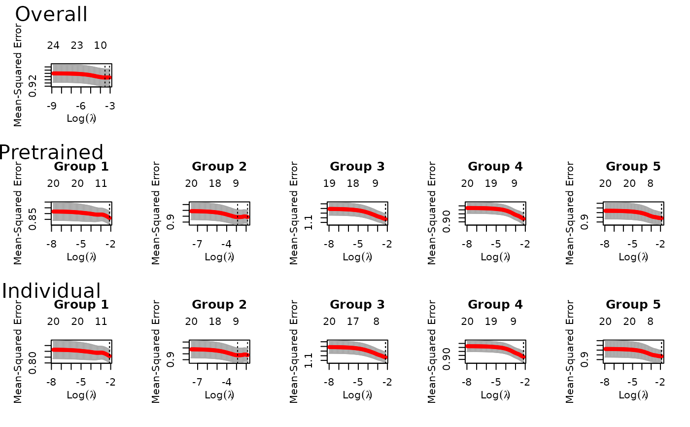predict(fit, xtest, groupstest) # to predict on new data
#> 
#> Call:  
#> predict.ptLasso(object = fit, xtest = xtest, groupstest = groupstest) 
#> 
#> 
#> 
#> alpha =  0.5 
#> 
#> Support size:
#>                                       
#> Overall    3                          
#> Pretrain   9 (0 common + 9 individual)
#> Individual 9                          
predict(fit, xtest, groupstest, ytest=ytest) # if ytest is included, we also measure performance
#> 
#> Call:  
#> predict.ptLasso(object = fit, xtest = xtest, groupstest = groupstest,  
#>     ytest = ytest) 
#> 
#> 
#> alpha =  0.5 
#> 
#> Performance (Mean squared error):
#> 
#>            allGroups  mean group_1 group_2 group_3 group_4 group_5       r^2
#> Overall        1.141 1.141   1.098   1.136   1.313   1.043   1.115 -0.003342
#> Pretrain       1.149 1.149   1.100   1.182   1.308   1.041   1.116 -0.010747
#> Individual     1.149 1.149   1.100   1.182   1.308   1.041   1.116 -0.010818
#> 
#> Support size:
#>                                       
#> Overall    3                          
#> Pretrain   9 (0 common + 9 individual)
#> Individual 9                          

# When we trained our model, we used "lambda.1se" in the first stage of pretraining by default.
# This is a necessary choice to make during model training; we need to select the model
# we want to use to define the offset and penalty factor for the second stage of pretraining.
# We could instead have used "lambda.min":
fit = ptLasso(x, y, groups = groups, alpha = 0.5, family = "gaussian", type.measure = "mse",
              overall.lambda = "lambda.min")

# We can use the 'relax' option to fit relaxed lasso models:
fit = ptLasso(x, y, groups = groups, alpha = 0.5,
              family = "gaussian", type.measure = "mse",
              relax = TRUE)

# As we did for lambda, we may want to specify the choice of gamma for stage one
# of pretraining. (The default is "gamma.1se".)
fit = ptLasso(x, y, groups = groups, alpha = 0.5,
              family = "gaussian", type.measure = "mse",
              relax = TRUE, overall.gamma = "gamma.min")

# In practice, we may want to try many values of alpha.
# alpha may range from 0 (the overall model with fine tuning) to 1 (the individual models).
# To choose alpha, you may either (1) run ptLasso with different values of alpha
# and measure performance with a validation set, or (2) use cv.ptLasso.


# Now, we are ready to simulate slightly more realistic data.
# This continuous outcome example has k = 5 groups, where each group has 200 observations.
# There are scommon = 10 features shared across all groups, and
# sindiv = 10 features unique to each group.
# n = 1000 and p = 120 (60 informative features and 60 noise features).
# The coefficients of the common features differ across groups (beta.common).
# In group 1, these coefficients are rep(1, 10); in group 2 they are rep(2, 10), etc.
# Each group has 10 unique features, the coefficients of which are all 3 (beta.indiv).
# The intercept in all groups is 0.
# The variable sigma = 20 indicates that we add noise to y according to 20 * rnorm(n). 
set.seed(1234)
k=5
class.sizes=rep(200, k)
scommon=10; sindiv=rep(10, k)
n=sum(class.sizes); p=2*(sum(sindiv) + scommon)
beta.common=3*(1:k); beta.indiv=rep(3, k)
intercepts=rep(0, k)
sigma=20
out = gaussian.example.data(k=k, class.sizes=class.sizes,
                            scommon=scommon, sindiv=sindiv,
                            n=n, p=p,
                            beta.common=beta.common, beta.indiv=beta.indiv,
                            intercepts=intercepts, sigma=20)
x = out$x; y=out$y; groups = out$group

outtest = gaussian.example.data(k=k, class.sizes=class.sizes,
                                scommon=scommon, sindiv=sindiv,
                                n=n, p=p,
                                beta.common=beta.common, beta.indiv=beta.indiv,
                                intercepts=intercepts, sigma=20)
xtest=outtest$x; ytest=outtest$y; groupstest=outtest$groups

fit = ptLasso(x, y, groups = groups, alpha = 0.5, family = "gaussian", type.measure = "mse")
plot(fit) # to see all of the cv.glmnet models trained

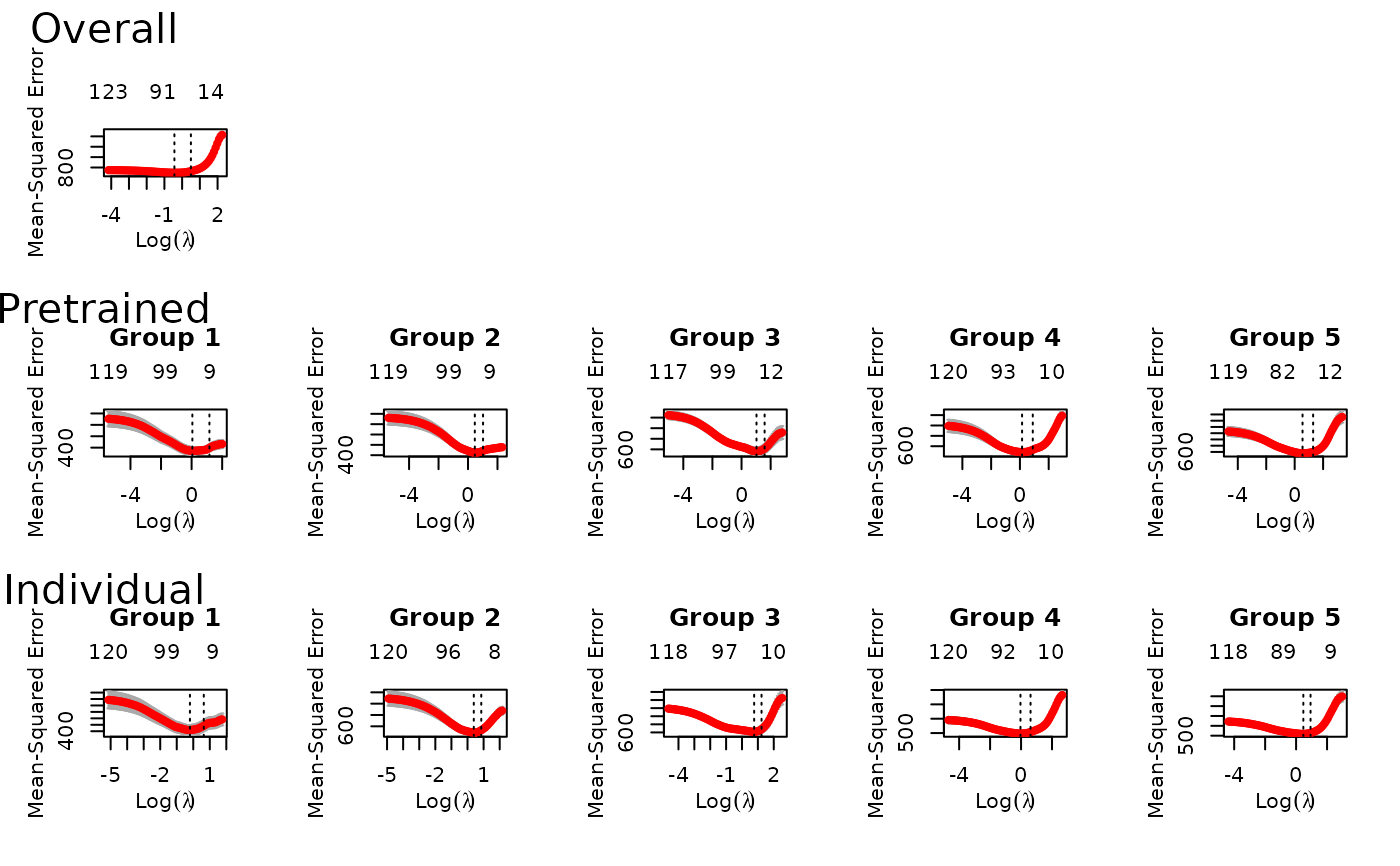predict(fit, xtest, groupstest, ytest=ytest)
#> 
#> Call:  
#> predict.ptLasso(object = fit, xtest = xtest, groupstest = groupstest,  
#>     ytest = ytest) 
#> 
#> 
#> alpha =  0.5 
#> 
#> Performance (Mean squared error):
#> 
#>            allGroups  mean group_1 group_2 group_3 group_4 group_5    r^2
#> Overall        755.7 755.7   836.0   554.9   565.4   777.9  1044.0 0.5371
#> Pretrain       503.2 503.2   550.6   443.3   553.5   505.6   462.9 0.6918
#> Individual     532.8 532.8   584.1   443.2   567.2   550.5   518.9 0.6736
#> 
#> Support size:
#>                                          
#> Overall    64                            
#> Pretrain   94 (21 common + 73 individual)
#> Individual 109                           

# Now, we repeat with a binomial outcome.
# This example has k = 3 groups, where each group has 100 observations.
# There are scommon = 5 features shared across all groups, and
# sindiv = 5 features unique to each group.
# n = 300 and p = 40 (20 informative features and 20 noise features).
# The coefficients of the common features differ across groups (beta.common),
# as do the coefficients specific to each group (beta.indiv).
set.seed(1234)
k=3
class.sizes=rep(100, k)
scommon=5; sindiv=rep(5, k)
n=sum(class.sizes); p=2*(sum(sindiv) + scommon)
beta.common=list(c(-.5, .5, .3, -.9, .1), c(-.3, .9, .1, -.1, .2), c(0.1, .2, -.1, .2, .3))
beta.indiv = lapply(1:k, function(i)  0.9 * beta.common[[i]])

out = binomial.example.data(k=k, class.sizes=class.sizes,
                            scommon=scommon, sindiv=sindiv,
                            n=n, p=p,
                            beta.common=beta.common, beta.indiv=beta.indiv)
x = out$x; y=out$y; groups = out$group

outtest = binomial.example.data(k=k, class.sizes=class.sizes,
                                scommon=scommon, sindiv=sindiv,
                                n=n, p=p,
                                beta.common=beta.common, beta.indiv=beta.indiv)
xtest=outtest$x; ytest=outtest$y; groupstest=outtest$groups

fit = ptLasso(x, y, groups = groups, alpha = 0.5, family = "binomial", type.measure = "auc")
plot(fit) # to see all of the cv.glmnet models trained

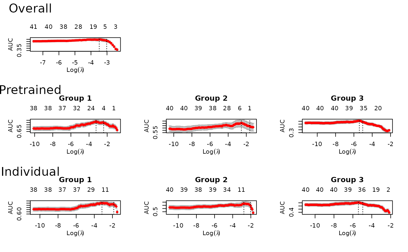predict(fit, xtest, groupstest, ytest=ytest)
#> 
#> Call:  
#> predict.ptLasso(object = fit, xtest = xtest, groupstest = groupstest,  
#>     ytest = ytest) 
#> 
#> 
#> alpha =  0.5 
#> 
#> Performance (AUC):
#> 
#>            allGroups   mean wtdMean group_1 group_2 group_3
#> Overall       0.5990 0.5963  0.5963  0.6006  0.6772  0.5112
#> Pretrain      0.6442 0.6631  0.6631  0.6965  0.7752  0.5177
#> Individual    0.6429 0.6580  0.6580  0.6948  0.7607  0.5186
#> 
#> Support size:
#>                                         
#> Overall    8                            
#> Pretrain   40 (3 common + 37 individual)
#> Individual 40                           

if (FALSE) { # \dontrun{
### Model fitting with parallel = TRUE
require(doMC)
registerDoMC(cores = 4)
fit = ptLasso(x, y, groups = groups, family = "gaussian", type.measure = "mse", parallel=TRUE)
} # }

# Multiresponse pretraining:
# Now let's consider the case of a multiresponse outcome. We'll start by simulating data:
set.seed(1234)
n = 1000; ntrain = 500;
p = 500
sigma = 2
     
x = matrix(rnorm(n*p), n, p)
beta1 = c(rep(1, 5), rep(0.5, 5), rep(0, p - 10))
beta2 = c(rep(1, 5), rep(0, 5), rep(0.5, 5), rep(0, p - 15))

mu = cbind(x %*% beta1, x %*% beta2)
y  = cbind(mu[, 1] + sigma * rnorm(n), 
           mu[, 2] + sigma * rnorm(n))
cat("SNR for the two tasks:", round(diag(var(mu)/var(y-mu)), 2), fill=TRUE)
#> SNR for the two tasks: 1.6 1.44
cat("Correlation between two tasks:", cor(y[, 1], y[, 2]), fill=TRUE)
#> Correlation between two tasks: 0.5164748

xtest = x[-(1:ntrain), ]
ytest = y[-(1:ntrain), ]

x = x[1:ntrain, ]
y = y[1:ntrain, ]

fit = ptLasso(x, y, type.measure = "mse", use.case = "multiresponse")
plot(fit)  # to see all of the cv.glmnet models trained

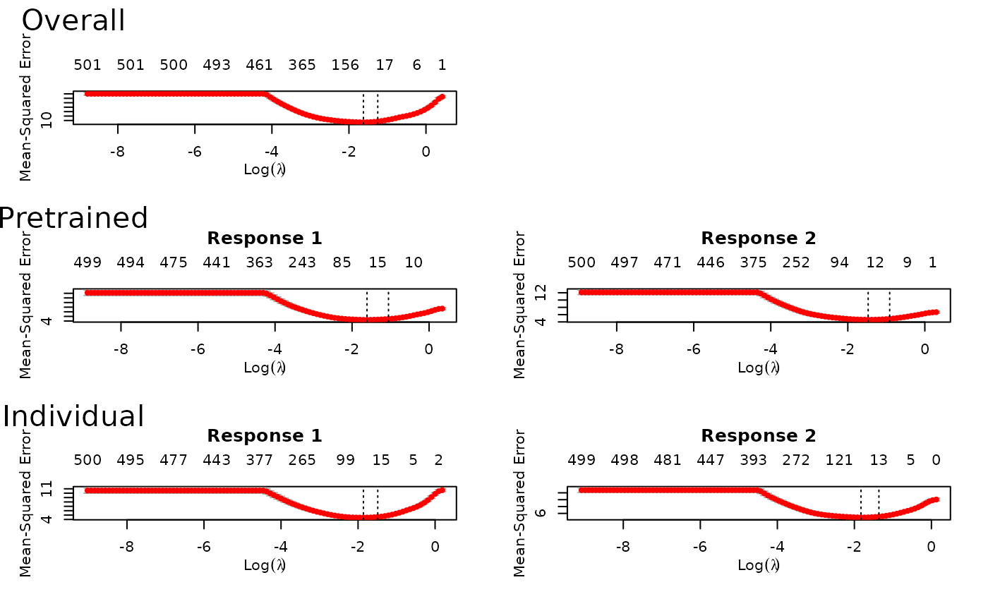predict(fit, xtest) # to predict with new data
#> 
#> Call:  
#> predict.ptLasso(object = fit, xtest = xtest) 
#> 
#> 
#> alpha =  0.5 
#> 
#> Support size:
#>                                          
#> Overall    57                            
#> Pretrain   29 (19 common + 10 individual)
#> Individual 80                            
predict(fit, xtest, ytest=ytest) # if ytest is included, we also measure performance
#> 
#> Call:  
#> predict.ptLasso(object = fit, xtest = xtest, ytest = ytest) 
#> 
#> 
#> 
#> alpha =  0.5 
#> 
#> Performance (Mean squared error):
#> 
#>            allGroups  mean response_1 response_2
#> Overall        9.394 4.697      4.227      5.168
#> Pretrain       9.022 4.511      4.144      4.878
#> Individual     9.465 4.733      4.243      5.222
#> 
#> Support size:
#>                                          
#> Overall    57                            
#> Pretrain   29 (19 common + 10 individual)
#> Individual 80                            
# By default, we used lambda = "lambda.min" to measure performance.
# We could instead use lambda = "lambda.1se":
predict(fit, xtest, ytest=ytest, s="lambda.1se")
#> 
#> Call:  
#> predict.ptLasso(object = fit, xtest = xtest, ytest = ytest, s = "lambda.1se") 
#> 
#> 
#> 
#> alpha =  0.5 
#> 
#> Performance (Mean squared error):
#> 
#>            allGroups  mean response_1 response_2
#> Overall        9.879 4.940      4.387      5.492
#> Pretrain       9.481 4.740      4.210      5.271
#> Individual     9.965 4.983      4.341      5.624
#> 
#> Support size:
#>                                         
#> Overall    19                           
#> Pretrain   19 (19 common + 0 individual)
#> Individual 27                           

# We could also use the glmnet option relax = TRUE:
fit = ptLasso(x, y, type.measure = "mse", relax = TRUE, use.case = "multiresponse")

# Time series pretraining
# Now suppose we have time series data with a binomial outcome measured at 3 different time points.
set.seed(1234)
n = 600; ntrain = 300; p = 50
x = matrix(rnorm(n*p), n, p)

beta1 = c(rep(0.5, 10), rep(0, p-10))
beta2 = beta1 + c(rep(0, 10), runif(5, min = 0, max = 0.5), rep(0, p-15))
beta3 = beta1 + c(rep(0, 10), runif(5, min = 0, max = 0.5), rep(.5, 5), rep(0, p-20))

y1 = rbinom(n, 1, prob = 1/(1 + exp(-x %*% beta1)))
y2 = rbinom(n, 1, prob = 1/(1 + exp(-x %*% beta2)))
y3 = rbinom(n, 1, prob = 1/(1 + exp(-x %*% beta3)))
y = cbind(y1, y2, y3)

xtest = x[-(1:ntrain), ]
ytest = y[-(1:ntrain), ]

x = x[1:ntrain, ]
y = y[1:ntrain, ]

fit =  ptLasso(x, y, use.case="timeSeries", family="binomial", type.measure = "auc")
plot(fit)

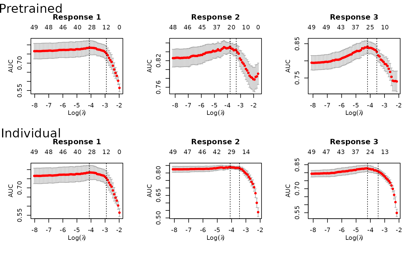predict(fit, xtest, ytest=ytest)
#> 
#> Call:  
#> predict.ptLasso(object = fit, xtest = xtest, ytest = ytest) 
#> 
#> 
#> 
#> alpha =  0.5 
#> 
#> Performance (AUC):
#> 
#>              mean response_1 response_2 response_3
#> Pretrain   0.8194     0.8194     0.8035     0.8354
#> Individual 0.7997     0.8194     0.7691     0.8106
#> 
#> Support size:
#>                                          
#> Pretrain   43 (26 common + 17 individual)
#> Individual 47                            

# The glmnet option relax = TRUE:
fit = ptLasso(x, y, type.measure = "auc", family = "binomial", relax = TRUE,
              use.case = "timeSeries")
plot(fit)

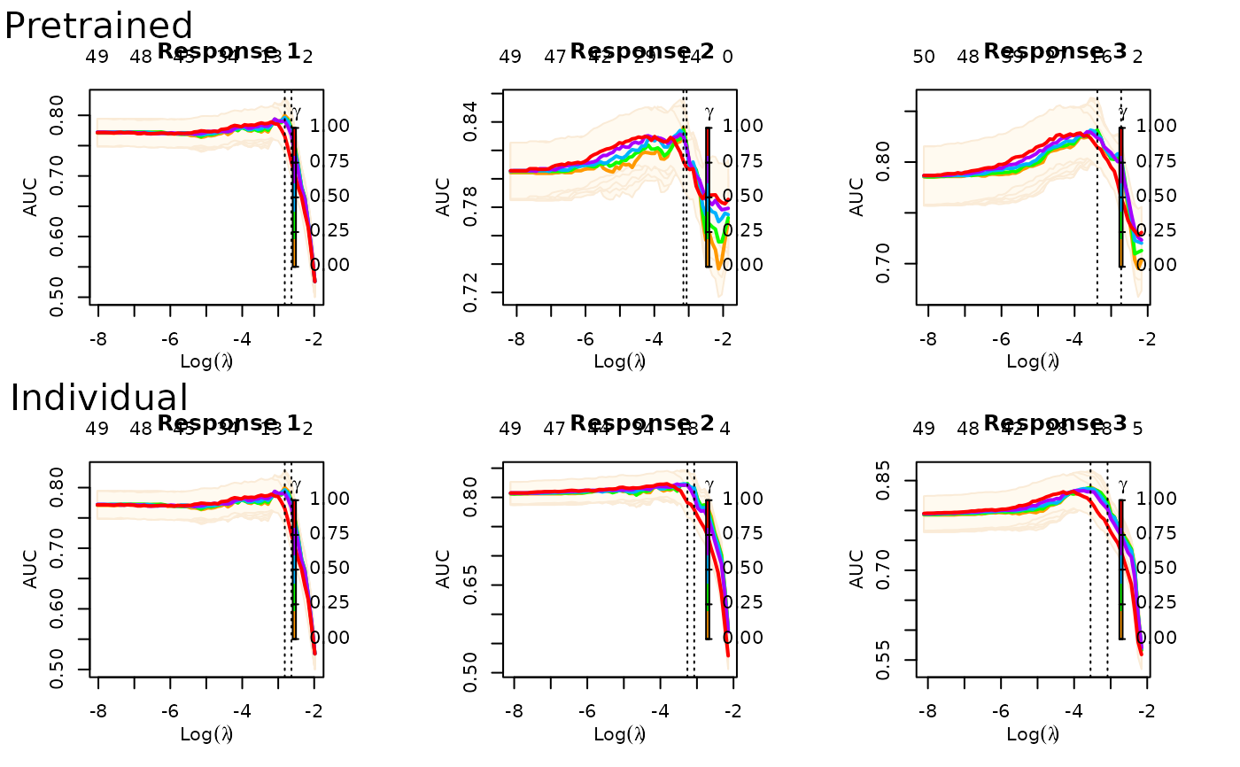predict(fit, xtest, ytest=ytest)
#> 
#> Call:  
#> predict.ptLasso(object = fit, xtest = xtest, ytest = ytest) 
#> 
#> 
#> 
#> alpha =  0.5 
#> 
#> Performance (AUC):
#> 
#>              mean response_1 response_2 response_3
#> Pretrain   0.8123     0.8298     0.7818     0.8252
#> Individual 0.8018     0.8298     0.7647     0.8110
#> 
#> Support size:
#>                                          
#> Pretrain   26 (12 common + 14 individual)
#> Individual 29